Step 1 - Your Budget Entry Sheet

This is where you'll plan your income & expenses each month. The best way to do this is estimate income & expenses for the year, then before the start of each month, go through and make your estimates more precise.

1. First off, double click on the sheet name at the bottom and enter "Budget Entry".
2. In B2 & C2, put "Category" & "Sub-Category"
3. Then in D2 through O2 add your month titles i.e. "Jan", "Feb", "Mar", etc.
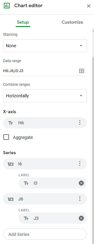
4. In P2 & Q2, put "Totals" & "Income?"
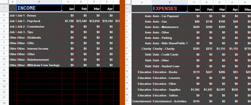
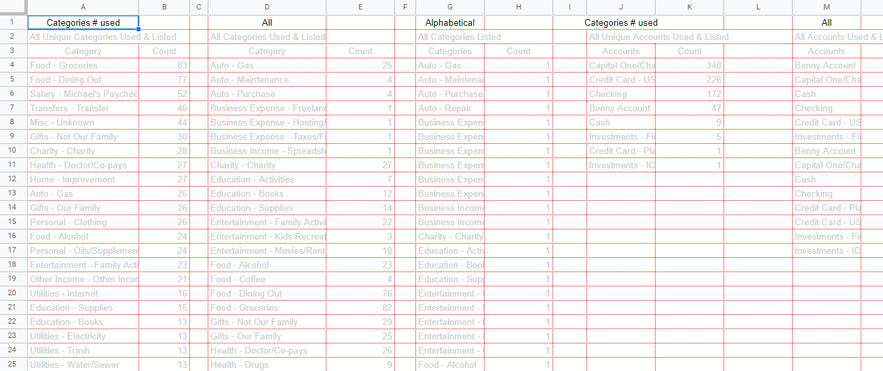
5. Column B will hold your income and expense categories such as your "Food", "Housing", "Utilities", "Salary". The sub-categories in column c will be a little more specific like "Groceries", "Dining Out", "Gas", "Rent", etc. Start with my sample categories or add your own.
6. Next, in A3 add the formula

   =if(B3<>"",CONCATENATE(B3," - ",C3),"")

• This formula looks in column B to see if it's blank, if it is it stays blank, if there is a value in B, then it puts "B's value - C's value"
7. After pasting the formula in A3, hit enter, then highlight A3 again. Drag the little blue box in the bottom right down about 150 rows.
8. Now right click on the column A header and "hide column".
9. Here's a little word of encouragement...."Good job so far" ;)
10. Next, paste this formula into P3 and drag it down 150 rows:

    =if(SUM(D3:O3)>0,SUM(D3:O3),"")

11. Highlight Q3, then click the menu "Data --> Data validation". Set the Criteria to "List of items" and then put "Purchase,Income" as the list. Make sure "Show dropdown list in cell" is checked and the other options don't matter. Click "Save".
12. Copy Q3, highlight the rest of column Q (Shift + Ctrl + ↓) and paste.
13. Lastly, put "Budgeted Saving/Deficit in C1"
14. Then put this formula in D1

    =sumif($Q$3:$Q,"Income",D3:D) - sumif($Q$3:$Q,"Purchase",D3:D)

15. And drag the little blue box across all the way to P1

Alright, that's our first sheet. Nicely down!

Step 2 - Accts Sheet

This sheet holds all of your accounts, checking, savings, investment, credit card, etc. You could even put your mortgage or other assets. It'll tally everything up and show total value of your accounts.

1. Start by adding a new sheet. Click the little plus sign in the bottom left of your window
2. Next, double click the new sheet named "Sheet2" at the bottom and entering "Accts".
3. To build the Accts sheet, we'll make one account, then copy and paste it down for a total of 12 accounts. You can go further if you need more than 12.
4. Start by putting your first account name in A2, then "Statement Date" in B2, "Starting Balance" in C2 and "Expenses", "Income", "Credits", and "Ending Balance" in D, E, F, and G
5. Highlight B3:B15 and change the background to a color that will help you know this is a cell you need to enter data into. Then click the "Format" menu click "Number", then click "Date".
6. In C4 put this formula to populate last month's ending balance as this month's Starting Balance

   =if(B4="","",G3)

7. Drag that formula down through C15.
8. Next, highlight D3:F15 and make it the same color background as column B but this time, under the Format menu select Number --> Currency.
9. Copy this format and paste it on C3.
10. Then at G3 paste the following formula to get the month's ending balance:

    =if(B3<>"",C3+D3+E3+F3,"")

11. Drag the blue box for G3 down to G15
12. Do any formatting you want to this account now, because we're about to duplicate it for the rest of the accounts.
13. To duplicate the account, highlight A1:G15, grab the little blue box at the bottom right and drag it down to G180.
14. The names you put in column A will appear in other dropdown menus throughout the spreadsheet, so nick names work but don't put other notes or things in column A.
15. Next, we'll make the summary box which gives you an idea which accounts need to be reconciled and what your balance is across all accounts.
16. Highlight I1:K1 and click the "Merge Cells" button. Then type "All Accounts".
17. In I2, J2, and K2 put "Month", "Balance", and "# Accts Reporting".
18. In I3:I14 you'll put "Jan", "Feb", etc.
19. Put this formula in J3. It will add all of the account's balances for each month

    =if((G214+G199+G184+G169+G154+G139+G124+G109+G94+G79+G64+G49+G34+G19+G4)=0,"",G214+G199+G184+G169+G154+G139+G124+G109+G94+G79+G64+G49+G34+G19+G4)

20. Then drag that cell's little blue box down to J14.
21. Lastly put this formula in K3. It will count how many accounts have values, meaning, they've been reconciled:

    =if(count(G214,G199,G184,G169,G154,G139,G124,G109,G94,G79,G64,G49,G34,G19,G4)=0,"",count(G214,G199,G184,G169,G154,G139,G124,G109,G94,G79,G64,G49,G34,G19,G4))

22. Then drag that cell's little blue box down to K14.
23. I don't love how bulky these formulas are and how they require nasty manual updates if you need to go beyond 12 accounts, so if anyone knows a better way to do this, lmk.
24. Last thing, select J3, click "Data" → "Named ranges" then name J3 "StartingBalance"

And that's the Accts sheet. We're on a roll now!

Step 3 - Transactions Sheet

Once we are done with the Complete Elite Spreadsheet, we won't need to interact with the Transactions sheet very much. But for now, this is where we'll put purchases and income transactions.

1. Start by, changing the sheet name to "Transactions".
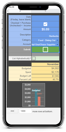
2. Then in A1 and all the way through H1, put the following values: "TransactionID", "Cleared", "Date", "Purchase or Income", "Amount", "Description", "Category", "Account".
3. Select B2, then click the menu "Data --> Data validation". Set the Criteria to "List of items" and then put "Y" as the list. Make sure "Show dropdown list in cell" is checked and the other options don't matter. Click "Save".
4. Copy B2 then select the rest of B (Shift + Ctrl + ↓) and paste.

That's it for the Transaction sheet!

Step 1 - Income & Expenses Sheets

You won't use these sheets very much, but they are important to hold your income and expenses through the year.

1. Start by naming this sheet "Income".
2. Then again, put "Income" in B1.
3. Then in C1 & D1 put 1/1/(current year) & 2/1/(current year). You can format these as dates, or under Format --> Number --> More Formats --> Custom date and time formats, you can select the abbreviated month as I've did.
4. Highlight those two cells and drag the little blue box across to N1.
5. In O1 & P1 put "Total" and "Average" respectively.
6. Next paste the following formula in A2

   =query('Budget Entry'!$A$3:$Q,"Select B, A Where Q = 'Income'",0)

• That looks at the Budget Entry sheet and grabs income categories and Categories together with Sub-Categories and lists all of them.
7. Now, put the following formula in C2

   =if(B2="","",sum(iferror(filter(Transactions!$E$2:$E, month(Transactions!$C$2:$C) = month(C$1), Transactions!$G$2:$G = $B2),0)))

• This pulls all of the transactions from the Transactions sheet that match what's in column B and adds them together if they occurred during the month listed in C1.
8. Now drag that formula down to the bottom of the sheet (this sheet doesn't need that many rows).
9. Next, with C2 through the rest of C highlighted (C2:C), drag the little blue box over to column N.
10. In O2 put the formula

    =if(B2="","",sum(C2:N2))

11. In P2 put the formula

    =if(B2="","",average(C2:N2))

12. Highlight O2 and P2 then drag the blue box down to the bottom of your rows.
13. To test if it is working, put a test transaction into the Transaction sheet using a value from column B as the transaction's category and a date anytime during this year. The value should show up in the correct row and column.
14. If it looks good, click on the little arrow next to the name of the sheet, then click Duplicate.
15. Rename the duplicate sheet by double clicking its name and type "Expenses".
16. Then on the "Expenses" sheet go to the formula in A2 and change 'Income' to 'Purchase'...this is a fun part...poof, the Expenses sheet is finished

Wooo! You made it through the first step of Lesson 2!

Step 2 - Average Spending & Graphs

This sheet tells you how your year is going financially. The graphs we're about to build display transaction data, not budget amounts. The Main graph is a two-axis graph with Income and Expenses on the left, Y-axis and Account Total Balance on the right. This is a pseudo-net worth graph.

1. Up to this point, everything we've built works for everyone. This sheet will require you to slightly customize the sheet to your needs. I'm going to walk you through a couple choices here.
2. The basic thing is, how many different sources of income do you want to track? For me, I have 10 and that is more than enough for me. If you have more sources of income, you'll need to change a couple formulas to meet your needs.
3. We are going to start by creating a new sheet and naming it "Graphs".
4. Go down to B57 (if you have more than 10 sources of income go further down).
5. Type in "Expenses".
6. In A59 put

   =ArrayFormula(iferror(match(B59:B,Expenses!A:A,0)))

7. This should list all of your expense categories.
8. We are going to list the various month across row 58, so you can either type them in, or put the following formula in C58 and drag it to N58

   =Expenses!C1

9. Ok, now to populate the values...in C59 put

   =if(isblank($B59),"", sumif(Expenses!$A:$A,$B59,Expenses!C:C))

10. Drag that formula to the bottom of the C column.
11. Now, with C58:C highlighted, drag that little blue box over to the N column.
12. In O59 put

    =if(isblank($B59),"", sum(C59:N59))

13. And in P59 put

    =if(isblank($B59),"", average(C59:N59))

14. Highlight both of those cells and drag them to the bottom of your sheet.
15. Ok, now let's do Income. Head up to B44 and type "Income". Technically, this section is optional, as we have what we need on the Income sheet, however, I found this easier than mapping the graphs we'll do next to multiple sheets.
16. Let's put the same Months across the top, so in C45 put the following formula in and drag it all the way to column P

    =C58

17. At this point you have a choice, If you want to see your income by category like expenses, just repeat the expenses instructions but pull from the Income sheet instead of the Expenses sheet.
18. For me, I have a lot more expense categories than income categories. So I'm going to show you how to display your income sub-categories here.
19. In B46 put the formula

    =arrayformula(unique(Income!B:B))

20. In A45, you are going to put "Row #".
21. There are a few ways to skin this cat...I chose this one.
22. In C46 put this formula

    =if(not(isblank(A46)), indirect("Income!c"&A46&":p"&A46),"")

23. Drag that formula down to C55, and you should have all months populated with income. Pretty cool huh?
24. Next up, we're going to sum all income and expenses, calculate a net saves or deficit for each month and add or subtract that from your overall starting balance.
25. So go up to B36 and type "Summary".
26. Let's daisy chain the column titles by putting the following formula in C 37 and dragging it to P37

    =c45

27. in B38, 39, 40 & 41 type "Income", "Expenses", "Net savings" & "Ending balance" respectively.
28. Now go up to C38 and put this formula

    =sum(C46:C56)

29. In C39 put

    =sum(C56:C)

30. In C40 put

    =C38-C39

31. In C41 put

    =StartingBalance+C40

32. Highlight C38:C41 and drag them across to column N.
33. In O38 put

    =sum(C38:N38)

34. In O39 put

    =sum(C39:N39)

35. And in O40 put

    =sum(C40:N40)

36. O41 gets

    =N41

37. Just four more formulas...
38. In P38 put

    =iferror(averageif(C38:N38, ">0", C38:N38), 0)

39. In P39 put

    =iferror(averageif(C39:N39, ">0", C39:N39), 0)

40. In P40 put

    =iferror(averageif(C40:N40, ">0", C40:N40), 0)

41. And in P41 put

    =iferror(averageif(C41:N41, ">0", C41:N41))

Wheeew! That's it for formulas and cells for this sheet, though we still need to create the graphs.

Income vs Spending + Total Balance Graph

OK, let's tackle the graphs now. First up, the more complex one. This graphs your monthly income vs monthly expenses on the left, Y-axis and the ending balance of all your accounts on the right, Y-axis.

1. Start by highlighting the range B37:N39
2. Next, click the menu "Insert" --> Chart
3. The Chart Editor should have popped up (if it didn't double click the chart).
4. The Chart Editor has two tabs, "Setup" & "Customize". Select "Setup".
5. Since we only highlighted Income & Expenses, we need to add another data range. So, click the grid button next under "Data range" - it should be to the right of the first range "B37:n39".
6. Click "Add another range" and type "B41:N41" click ok.
7. Now down below click "Add Series".
8. Select "Ending balance".
9. Now up at the top of the Chart Editor under "Chart type" select "Combo chart".
10. Next click "Customize" then delete whatever is under "Chart & axis titles" "Title text".
11. Click on "Series" and click where it says "Apply to all series" then select "Ending Balance".
12. Change "Type" from "Line" to "Area".
13. Then under where it says "Axis", change that from "Left axis" to "Right axis".
14. Click on "Series" again and select "Income" and change the "Type" from "Columns" to "Line".
15. The only other thing with this chart is to play with the colors, point shapes and whatever other aesthetics you want to mess with.

Average Monthly Income/Expenses Graphs

The average income and average expense charts are so much easier.

1. Adding the average monthly spend per category is pretty simple. Start by selecting B59 (or lower if you started your expenses table lower) and highlight the rest of column B - you should have all your categories highlighted.
2. Now, hold the CTRL (Command on a Mac) button and highlight P59:P.
3. You should have all of your categories (as well as blank category rows) & all of your averages highlighted.
4. Next, click the menu "Insert" --> Chart.
5. Play around with the appearance as you like and then do the same thing for income if you like.

The Graphs page is a little more of a few-times-per-year type of information. Now let's build a budget dashboard that will be useful every day.

Step 3 - Budget Dashboard

Dashboard Data

1. Like the Graphs sheet, we're going to build the data first, then the graphs.
2. Start in A1 with a simple "Year", then go to B1 and click the menu "Data" --> Data validation. List out the current years and next year - make sure "Show dropdown list in cell" is checked.
3. Next put "Month:" in A3 and highlight B3 and go back to "Data validation" and "Criteria: List of items" put

   Jan,Feb,Mar,Apr,May,Jun,Jul,Aug,Sep,Oct,Nov,Dec

4. C2 & C3 will get the following two formulas:

   =date(B1,month(B3&1),1)

   =EOMONTH(C2,0)

• You can hide these cells like I have with font color matching background color, or hide the whole column...up to you.
5. Now go over to L3 and put the following formula in it:

   =date(B1,month(B3&1),1)

   =QUERY('Budget Entry'!$A3:$Q,"SELECT B, A, Q, "&substitute(ADDRESS(2,MATCH($B$3,'Budget Entry'!$A$2:$O$2,0),4),2,"")&" where Q = 'Purchase'",0)

6. In P3 put:

   =ARRAYFORMULA(if(L3:L="","",if(O3:O>0,O3:O,0)))

7. In Q3 put:

   =sumifs(Transactions!E:E,Transactions!G:G,M3,Transactions!C:C,">="&$C$2,Transactions!C:C,"<="&$C$3)

8. In R3 put:

   =if(if(N3="Income",Q3-O3,O3-Q3)=0,"",if(N3="Income",Q3-O3,O3-Q3))

• This is a detailed look at your sub-categories budgeted values for the month selected in B3 together with actual expenses and the differences.
9. Now let's summarize that data down to the category level.
10. In H3 put this formula:

    =query($L$3:$R,"Select L, Sum(P), sum(Q) where L is not null and (P !=0 or Q != 0) group by L order by sum(P) desc label Sum(P) 'Budgeted', Sum(Q) 'Actual' ",0)

11. Then in K3 & K4 put "Remaining" and

    =iferror(if(I4="","",if(I4=0,(I4-J4)/J4,(I4-J4)/I4)),"")

12. Select K4 again and drag that little blue square in the bottom right down about 50 rows or so. If you have more than 50 categories...you might be too organized.
13. With your 50ish rows in column K highlighted, click the menu "Format" --> Conditional formatting. Then click "Add another rule"
14. Instead of "Single color" select "Color scale". Now, under "Preview" click "Default" and select the one you want. I find Red to White to Green to be the most intuitive - though I did have to change the white to work with my background color.
15. Now let's add up our budgeted & spending data by putting "Budget", "Actual" and "Overall" in I1, J1 and H2 respectively.
16. Then in I2 & J2 put these formulas:

    =sum(I4:I)

    =sum(J4:J)

17. Alright, 3 more formulas, then a bunch of charts.
18. In E2 put

    =I2-J2

19. In E3 put

    =(I2-J2)/I2

20. In F2 put

    =if(E3>0,"Budget Left","Over Budget")

21. Optional: Highlight F2:F3 and then click the Merge cells button.
22. The first graph will be an overall budget vs spending for the month, so highlight H1:J2 and click the "Insert" menu and select "Chart".
23. Format the chart how you like and position it where you want. I've used the left side of the sheet for mobile use.
24. Highlight H3:J4 and insert another chart.
25. For the rest of the charts, you are going to highlight H3:J3, then control click and highlight H5:J5 and insert another chart, then H3:J3, CTRL click H6:J6, etc. etc. etc.
26. In the Chart editor, I have H5 as the X-axis, and I value for Series 1 with I3 as it's label, a J value with J3 as it's label. Like this:

That's it for Lesson 2!

Step 1 - Data Sheet

This is a set-it and forget-it sheet. Once we're done here, you can drag this sheet all the way to the right and never look at it again.

We are going to query our budget entry sheet to get the a comprehensive list of sub-categories, we are going to query the transactions sheet to get a count of how many times each sub-category was used and then, we are going to put those two queries together.

Then we are going to do the same for Accounts.

1. Start by naming this sheet "data".
2. Then in G1 & G2, put "Alphabetical" & "All Categories Listed".
3. In G3 put:

   =QUERY('Budget Entry'!A3:A,"select A, 1 where A is not null order by A label A 'Categories', 1 'Count'",0)

4. Next, in D1 & D2, put "All" & "All Categories Used & Listed".
5. Then in D3 put:

   =ARRAYFORMULA(Unique({Query(Transactions!G2:G&{"",""},"select Col1, count(Col2) where Col1 != '' group by Col1 order by Col1 label Col1 'Category', count(Col2) 'Count'",0);G4:H}))

6. Now, in A1 & A2, put "# Used" & "All Unique Categories Used & Listed".
7. And finally, in A3 put:

   =sort(Query(D4:E, "select D, sum(E) where D != '' group by D label D 'Category', sum(E) 'Count'",0),2,false)

8. Ok, rapid fire for the Accounts...Ready, Set, Go!
9. Copy A1:G2 and paste it in J1, then go back and change "Categories" to "Accounts"
10. P3 gets

    =QUERY(Accts!A2:A,"select A, 1 where A is not null order by A label A 'Accounts', 1 'Count'",0)

11. M3 gets

    =ARRAYFORMULA(Unique({Query(Transactions!H2:H&{"",""},"select Col1, count(Col2) where Col1 != '' group by Col1 order by Col1 label Col1 'Accounts', count(Col2) 'Count'",0);P4:Q}))

12. J3 gets

    =sort(Query(M4:N, "select M, sum(N) where M != '' group by M label M 'Accounts', sum(N) 'Count'",0),2,false)

Alright. That is step 1!

Step 2 - Transaction Entry Form

Here we will build a sheet that functions like an input form to make it easy to record transactions when you are out and about.

1. Start by creating a new sheet and naming it "Transaction Entry"
2. Next, add labels - Put "Date (if today, leave blank)" in B2
3. Put "Checked = Purchase Unchecked = Income" in B3
4. B4 gets "Amount"
5. B5 gets "Description"
6. "Category" for B6
7. "Account" in B7
8. "Submit" goes in B8
9. And "List Alphabetically?"
10. Ok, now for the other column...Add a checkbox in C3, C8 and C10 by clicking "Insert" --> "Checkbox"
11. That's it for the top, it won't do anything until we add the code, but first, let's set up the snapshot below
12. We're going to grab our total budget for the current month by putting this formula in B24

    =QUERY('Budget Entry'!$A3:$Q,"SELECT sum("&substitute(ADDRESS(2,month(today())+3,4),2,"")&") where Q = 'Purchase'",0)

13. Then, we are going to grab the total expenses for the current month. Put this formula in C24

    =QUERY(Transactions!$C2:$E,"SELECT sum(E) where D = 'Purchase' and C >= date '"&text(eomonth(today(),-1)+1,"yyyy-mm-dd")&"' and C <= date '"&text(EOMONTH(eomonth(today(),-1)+1,0),"yyyy-mm-dd")&"'",0)

14. Alright, in B13, B14 and B16 put "Budgeted", "Spent" and "Percent Left".
15. And in B15 put:

    =if(C15>0,"Budget Left","Over Budget")

16. C12 gets:

    =text(today(),"MMMM")

17. C13 gets:

    =B25

18. C14 gets:

    =C25

19. C15 gets:

    =C13-C14

20. and C16 should be formatted as a percentage and put this formula in:

    =(C13-C14)/C13

21. Last thing before we put the code in...highlight B13:C14, click "Insert" --> "Chart"
22. Adjust that chart to fit and format accordingly.

Step 3 - Script for the Win!

Before we finish the last step, I'd like to say, I am proud of you for making it this far. If you are willing to put this much work in, I know you have the buy-in to stick to your budget and reach your financial goals.

If you are able and want to encourage me, my venmo is Michael-Shipe-1. Event a little bit is very encouraging ;)

We're going into the guts of Google Sheets here to create some scripts that Submit Transactions and List Accounts/Categories by use as well as alphabetically.

1. Here is where it gets good. First open the script editor by clicking "Tools" --> "Script editor".
2. Here is the code that takes your transaction data from the input form and records it in the Transactions sheet. Quick note, these scripts reference sheet names exactly, so if you run into any problems, double-check that the sheet names in this code match your sheet names:

   function submitData() {
     var ss        = SpreadsheetApp.getActiveSpreadsheet();
     var formSS    = ss.getSheetByName("Transaction Entry"); //Data entry Sheet
     var datasheet = ss.getSheetByName("Transactions"); // Destination Sheet
     var today     = formSS.getRange("C2").getValue(); // date
   
     // If they left the date cell blank, use today's date
     if ( today === "" ){
       today = Utilities.formatDate(new Date(), "GMT-5", "MM/dd/yyyy");
     }
   
     // See if the purchase checkbox is checked and set the 'purchase' variable accordingly
     var purchase = formSS.getRange("C3");
     if ( purchase.isChecked() ){
       purchase = "Purchase";
     } else {
       purchase = "Income";
     }
   
     // Set a confirmation message
     var msg1 = "Got it.";
   
     // Find the last transaction ID and create a transaction ID for this entry
     var lastId = datasheet.getRange(datasheet.getLastRow(),1).getValue();
     var newId = lastId + 1;
   
     // Grab the variables and input values from the sheet and hold them in an array called 'values'
     var values = [[newId,
                    "",
                    today,
                    purchase,
                    formSS.getRange("C4").getValue(),
                    formSS.getRange("C5").getValue(),
                    formSS.getRange("C6").getValue(),
                    formSS.getRange("C7").getValue()]];
   
     // Record the transaction data in the transaction sheet
     datasheet.getRange(datasheet.getLastRow()+1, 1, 1, 8).setValues(values);
   
     // Record the confirmation message
     formSS.getRange("C9").setValue(msg1);
   
     // Clear the form's content
     formSS.getRange("C2").clearContent();
     formSS.getRange("C4:C8").clearContent();
   }

3. Now, that "submidData" function needs to be triggered when we check the "submit" checkbox. So to do that, we'll need a server-side script listening for changes like the following. Put this code above the previous chunk:

   function onEdit(e){
     const rg = e.range; // the range changed
   
     // If the "range changed" is C8, then submit the data
     if(rg.getA1Notation() === "C8" && rg.isChecked()){
       submitData(); // run the submitData function
       rg.uncheck(); // clear the submit checkbox
     }
   
   }

4. One problem here is that this script is listening for changes in C8, regardless of which sheet you are on. So let's add an if statement checking that the active sheet is the Transaction Entry sheet. Let's also add a listener that looks for changes on C4 that clears the confirmation message so the cell is blank so it's ready to display another confirmation message. So update the onEdit function with this:

   function onEdit(e){
     const rg = e.range; // the range changed
     // Listening for changes on Transaction Entry sheet
     if(rg.getSheet().getName() === "Transaction Entry"){
       // Clear confirmMsg
       if(rg.getA1Notation() === "C4"){
         var spreadsheet = SpreadsheetApp.getActive();
         spreadsheet.getRange('\'Transaction Entry\'!C9').clearContent();
       }
   
       // If the "range changed" is C8, then submit the data
       if(rg.getA1Notation() === "C8" && rg.isChecked()){
         submitData(); // run the submitData function
         rg.uncheck(); // clear the submit checkbox
       }
     }
   }

5. So, we are going to build two functions, mostUsed() & alpha() to grab our categories and accounts from the data sheet we built in step 1. I've got these functions sitting just above the submitData function.

   function mostUsed() {
     // Categories
     var spreadsheet = SpreadsheetApp.getActive();
     // create a new data validation in Transaction Entry C6 based off A4:A in the data sheet
     spreadsheet.getRange('\'Transaction Entry\'!C6').setDataValidation(SpreadsheetApp.newDataValidation()
     .setAllowInvalid(true)
     .requireValueInRange(spreadsheet.getRange('data!$A$4:$A'), true)
     .build());
   
     // Accounts
     var spreadsheet = SpreadsheetApp.getActive();
     // create a new data validation in C7 for accounts based off the J column in Data
     spreadsheet.getRange('\'Transaction Entry\'!C7').setDataValidation(SpreadsheetApp.newDataValidation()
     .setAllowInvalid(true)
     .requireValueInRange(spreadsheet.getRange('data!$J$4:$J'), true)
     .build());
   };
   
   function alpha() {
     // Categories
     var spreadsheet = SpreadsheetApp.getActive();
     // build the same data validations but based off different columns in data
     spreadsheet.getRange('\'Transaction Entry\'!C6').setDataValidation(SpreadsheetApp.newDataValidation()
     .setAllowInvalid(true)
     .requireValueInRange(spreadsheet.getRange('data!$G$4:$G'), true)
     .build());
   
     // Accounts
     var spreadsheet = SpreadsheetApp.getActive();
     // build the same data validations but based off different columns in data
     spreadsheet.getRange('\'Transaction Entry\'!C7').setDataValidation(SpreadsheetApp.newDataValidation()
     .setAllowInvalid(true)
     .requireValueInRange(spreadsheet.getRange('data!$P$4:$P'), true)
     .build());
   };

6. Now we are going to add a simple if statement to our onEdit function that says, if the "List Alphabetically" box is checked, run the alpha function, if it is unchecked, run the mostUsed function. Put it just inside the last closing curly bracket "}" of the onEdit function

       // Sort categories and accounts
       if(rg.getA1Notation() === "C10" && rg.isChecked()){
         alpha();
       } else {
         mostUsed();
       }

Great job! You are nearing the finish line. One. More. Step.

Step 4 - Reconciling Magic

This page is awesome and I'll tell you why, This page makes reconciling back accounts SO much faster. You put in your statement details into the account sheet, then pull that account up on this page and displays all of the transactions for that account for the statement dates. Not only that, but you can mark them cleared from this one screen.

1. This might look complicated, but let's break it down
2. First in C1 put "Account:"
3. Then highlight D1 and click "Data" → "Data validation".
4. For "Criteria:" select "List from a range" and make that range Accts!A:A. Make sure "Show dropdown list" is checked and click save.
5. Next highlight D1:F1 and click the "Merge cells" button.
6. Now put "Start Date:" in B2 and "Prev. Balance" in B3
7. "End Date:" goes in E2 and "New Balance" goes in E3
8. Now, this complicated formula goes in C2 and takes the account listed in D1 and finds it on your Accts sheet. It then grabs the second to last statement date

   =INDEX(INDIRECT("Accts!B"&MATCH(D1,Accts!A:A, 0)+1&":B"&(MATCH(D1,Accts!A:A, 0)+1)+11), MATCH(99^99,INDIRECT("Accts!B"&MATCH(D1,Accts!A:A, 0)+1&":B"&(MATCH(D1,Accts!A:A, 0)+1)+11), 1)-1)

9. This formula does a similar thing but grabs the starting balance. It goes in C3

   =INDEX(INDIRECT("Accts!c"&MATCH(D1,Accts!A:A, 0)+1&":c"&(MATCH(D1,Accts!A:A, 0)+1)+11), MATCH(99^99,INDIRECT("Accts!c"&MATCH(D1,Accts!A:A, 0)+1&":c"&(MATCH(D1,Accts!A:A, 0)+1)+11), 1))

10. Put this one in F2 as it gets the statment's end date

    =INDEX(INDIRECT("Accts!B"&MATCH(D1,Accts!A:A, 0)+1&":B"&(MATCH(D1,Accts!A:A, 0)+1)+11), MATCH(99^99,INDIRECT("Accts!B"&MATCH(D1,Accts!A:A, 0)+1&":B"&(MATCH(D1,Accts!A:A, 0)+1)+11), 1))

11. And you probably guessed it, this one goes in F3

    =INDEX(INDIRECT("Accts!G"&MATCH(D1,Accts!A:A, 0)+1&":G"&(MATCH(D1,Accts!A:A, 0)+5)+11), MATCH(99^99,INDIRECT("Accts!G"&MATCH(D1,Accts!A:A, 0)+1&":G"&(MATCH(D1,Accts!A:A, 0)+1)+11), 1))

12. Next let's put our column headers up for our expenses.
13. Starting in B6 and going over to I6 put "Trans. ID", "Cleared", "Date", "P/I", "Amount", "Description", "Category", "Account".
14. This formula rocks. It is going to grab all of the transactions for the selected account that fall between the start and end dates. Put this in B7

    =iferror(sort(query({filter(Transactions!$A$2:$H, Transactions!$C$2:$C > $C$2, Transactions!$C$2:$C <= $F$2, Transactions!$H$2:$H = $D$1,Transactions!$D$2:$D = "Purchase")},"select * WHERE Col3 Is Not NULL"),3,TRUE),"No Transactions Found")

15. Let's sum the total expenses by putting "Cleared Expenses / Debits" in D4 and this formula in D5

    =sumif(C7:C, "Y", F7:F)

16. Go to A7, click "Insert" → "Checkbox" the copy that check box from A7 and paste it to the bottom of the A column.
17. Now highlight A4 through the bottom of the I column, copy that and paste it on K4.
18. This will be our income side, so replace the formula in L7 with this one:

    =iferror(sort(query({filter(Transactions!$A$2:$H, Transactions!$C$2:$C > $C$2, Transactions!$C$2:$C <= $F$2, Transactions!$H$2:$H = $D$1,Transactions!$D$2:$D = "Income")},"select * WHERE Col3 Is Not NULL"),3,TRUE),"No Transactions Found")

19. We need one more formula to bring this together. When the formula in G5 reaches $0.00, your account is reconciled. It takes the account's starting balance - subtracts the purchases adds the income and then subtracts the account's ending balance

    =C3-D5+N5-F3

The very last thing is to edit our script so when you check or uncheck the checkboxes, it records them cleared on the transactions sheet and gets them counted here towards Reconciliation.

1. Go back to your script editor under "Tools". Remember how we added the sheet name "Transaction Entry" to the onEdit function so it would only run that function when you are modifying the specified cells on that sheet. It is time to find the end of "if(rg.getSheet().getName() === "Transaction Entry"){" and add an "else if" statement.
2. The easiest way to do this is just delete your whole onEdit function and replace it with

   function onEdit(e){
     const rg = e.range;
   
     // Listening for changes on Transaction Entry sheet
     if(rg.getSheet().getName() === "Transaction Entry"){
       // Clear confirmMsg
       if(rg.getA1Notation() === "C4"){
         var spreadsheet = SpreadsheetApp.getActive();
         spreadsheet.getRange('\'Transaction Entry\'!C9').clearContent();
       }
   
       // If the "range changed" is C8, then submit the data
       if(rg.getA1Notation() === "C8" && rg.isChecked()){
         submitData();
         rg.uncheck();
       }
   
       // If the "range changed" is C10, then submit the data
       if(rg.getA1Notation() === "C10" && rg.isChecked()){
         alpha();
       } else {
         mostUsed();
       }
     } else if (rg.getSheet().getName() === "Reconciling"){ // Listening for changes on Reconciling sheet
       // mark transaction as cleared from reconciling sheet to transaction sheet
       if(rg.getColumn() === 1 || 11){ // if the change is in column 1 or 11 (the ones with the check boxes)
         var spreadsheet = SpreadsheetApp.getActive();
         var row = rg.getRow();
         var col = rg.getColumn();
         var transId = SpreadsheetApp.getActiveSheet().getRange(row,col + 1);
         var id = transId.getValue(); // get the id of the transaction that was checked
   
         // insert 'y' in transactions sheet in the cell next to id
         var ss = SpreadsheetApp.getActiveSpreadsheet();
         var datasheet = ss.getSheetByName("Transactions"); // Destination Sheet
         var data = datasheet.getDataRange().getValues();
   
         // find the row with the id searching backwards through all transactions
         for(var i = data.length - 1; i >= 0; i--){
           if(data[i][0] == id){
             var row = (i+1)
             break;
           }
         }
   
         // add/remove 'Y' next to that transaction
         if(rg.isChecked()){
           datasheet.getRange(row,2).setValue('Y');
         } else {
           datasheet.getRange(row,2).setValue('');
         }
       }
   
       // Clear checkboxes on Reconciling sheet when account in D1 is changed
       if(rg.getA1Notation() === "D1"){
         var spreadsheet = SpreadsheetApp.getActive();
         spreadsheet.getRange('A7:A').clearContent();
         spreadsheet.getRange('K7:K').clearContent();
       }
     }
   }

That's it! You did it! Nice work!

Great job getting through this...I didn't know if anyone would take the time.

If this has been helpful for you and you want to say thanks, my venmo is Michael-Shipe-1.